|
Now that I am well started, it is time to tell you a bit about my project. This summer, 410 patients, all affected by gliomas (i.e brain tumours), had their DNA extracted to characterise their mutational status. Therefore, my internship goal is to amplify genes of interest (named IDH1, IDH2 and Tert [2,3]) by PCR to allow Sanger sequencing and then investigate potential mutations. Ultimately, I will carry out statistical analyses to estimate the impact of each mutation on survival and to compare my results with the available bibliography. Feel free to ask me anything about this project! 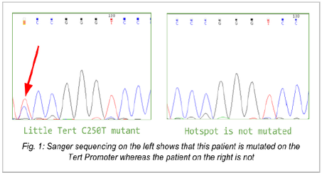 References:
[1] YouTube. (2017). Metallica & San Francisco Symphony Orchestra - Master Of Puppets. [online] Available at: https://www.youtube.com/watch?v=A39C6o6x-fU [Accessed 29 Mar. 2017]. [2] Labussière, M., Di Stefano, A., Gleize, V., Boisselier, B., Giry, M., Mangesius, S., Bruno, A., Paterra, R., Marie, Y., Rahimian, A., Finocchiaro, G., Houlston, R., Hoang-Xuan, K., Idbaih, A., Delattre, J., Mokhtari, K. and Sanson, M. (2014). TERT promoter mutations in gliomas, genetic associations and clinico-pathological correlations. British Journal of Cancer, 111(10), pp.2024-2032. [3] Boisselier, B., Gallego Perez-Larraya, J., Rossetto, M., Labussiere, M., Ciccarino, P., Marie, Y., Delattre, J. and Sanson, M. (2012). Detection of IDH1 mutation in the plasma of patients with glioma. Neurology, 79(16), pp.1693-1698. For a short-but-still-useful reminder of what a PCR is: YouTube. (2017). PCR - Polymerase Chain Reaction (IQOG-CSIC). [online] Available at: https://www.youtube.com/watch?v=iQsu3Kz9NYo [Accessed 29 Mar. 2017]. If you want to know more about Sanger sequencing, gold standard method to look for mutants: Thermofisher.com. (2017). Sanger Sequencing Method | Thermo Fisher Scientific. [online] Available at: https://www.thermofisher.com/fr/fr/home/life-science/sequencing/sanger-sequencing/sanger_sequencing_method.html# [Accessed 30 Mar. 2017].
7 Comments
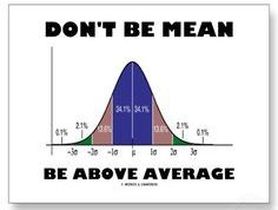 Fig.1: let's start with a bit of humour, shall we? Fig.1: let's start with a bit of humour, shall we? Relax and enjoy your flight on Biostatistics Airlines: First thing I’ve done while crossing path with medical biostatistics was… laughing. A mirthless laugh: those formulae were unintelligible. What I did not understand then was that, at our little level, the only thing we need is… knowing what we want! Indeed, each described situation can be reduced to a formula. In the previous post, we’ve seen that distributing patients into prognostic strata was possible by comparing two genes mutation status within different tumour types and their combined impact on prognostic. What is the prognostic here? Simply survival. What do we want? Simply knowing if Mr X with mutated A but wild-type (i.e the gene “normal” state) B will live longer than Mrs Y with both wild-type A and B. So let’s not forget that statistics can be easy to grasp if those concepts are explained with the right handle [1] and let’s slowly take one step after another to understand how survival analysis is made and can help us on our journey toward personalised medicine. First step: datum datum datum, dati, dato dato, DATA, DATA, DATA, datorum, datis datis We are all familiar with the first step of every statistical analysis: data collection. In the introduction, it is said that we are interested by survival: at a given time is a given patient dead or alive (yes, mathematics can be pretty cynical)? Some of you who already know a bit about statistics may ask why we do not use the classical models such as the Normal Law (Gaussian curve [2]) that allow easy interpretations. It is because survival do not follow classical distributions and events are often distributed as follows: several early events, some late events [3]. So survival analysis requires specific models. There are two “events” that can be observed: death or recurrence (i.e cancer comes back). Models use two variables linked to these events: i) overall survival: time between diagnostic and death or the last follow-up ii) progression free survival: time between the response to the treatment and the recurrence or the last follow-up Here “follow-up” means the time when you examine all the patients in your cohort. What is interesting is that this notion of follow-up is another point that makes survival analysis different from other models. If patients do not exhibit death nor recurrence, they are considered as “censored” in the study i.e they do not give objective data therefore classical models are not relevant either. The only thing you need to keep in mind is that censoring events follows specific rules [4]. Second step: “All Curves Are Beautiful” (Yvan Cornut) Now that we have our data, we have to put them into functions to model what we want. Two functions are used [3]: i) survival S(t) that represents the “cumulative non occurrence” i.e the the summed time a patient survived ii) hazard h(t) that represent the event occurrence at a given time t knowing that until t, the patient did not experience any events. Those function will be useful to plot survival curves, a way to represent survival in order to analyse it more easily. The most common way to do it is by using the Kaplan-Meier method: 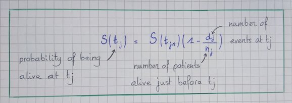 Fig.2: Formula for the KM Method. Relax, it is simpler than most of mathematical things we’ve done so far! 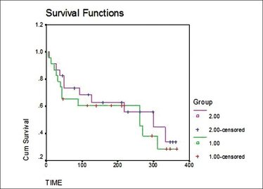 Fig.3: Kaplan-Meier curves, S(t) = f(t) Fig.3: Kaplan-Meier curves, S(t) = f(t) As initial conditions we have:
If you’re a cynical, you can plot [1-S(t)] vs. time to obtain death curves but let’s stay positive, after all, you’re still alive after the previous explanations :)
Next step: comparing your curves. Why? Because all differences are not significant. Huu... what? Let me be clearer: when you cook, it will be significantly different to add 10 more grams of butter than only one gram. Same thing for your survival curve: How big must be the difference so you can conclude that if Mr X with wt-B and mutated A live longer, everyone is more likely to also live longer? To do that, we use a test named log rank [6] and performed the same way as a χ² [5]. No, no, don’t go! I’ll be happy to develop in the comments for those who may be interested but let’s stop there on survival curves and take another step. Last-but-not-least step: what else? In the first blogpost, we saw that cancer was a multifactorial disorder with internal and external causing factors. Methods like the ones above (Kaplan Meier and log rank) are univariate. Hence the need for models that take into account the factors linked to the patient (remember: personalised approach) named cofounders or covariates and that allow to estimate clinically [7] (not statistically) the impact of the mutation status combined with those factors on the prognostic. There are two categories of models that differ by the way impact on the prognosis is conceived. In the Cox proportional hazard model that we will see below, each factor has a weight that influences the prognosis whereas in the Accelerated Failure Time model that will not further be detailed, each factor can shrink or stretches the survival time along the time-axis. Briefly, the Cox semi-parametric is a way to link event occurrences with the covariate set. It uses the following function of the hazard h(t): h(t) = h0(t) x exp(i=1pbi.xi) That can appear absolutely barbaric until you just know that p is the number of covariates you are considering (age at diagnosis, gender, other disorder…), x a given covariates and b its relative coefficient that weigh the hazard. Still following? Great! Here are some little precisions: i) h0(t) is a “basal hazard” that is very convenient because we do not have to assume that h(t) follows a given and known distribution ii) This model can only be applied under the assumption that all the risks are constant multiples. iii) exp(bi) is the risk ratio and allows to better understand the model: if b>0, h(t) increases therefore, if the risk increases, the survival time decreases. Thus we have a negative correlation between risk ratios and survival Now you know! Congratulations, you have succeeded in following statistical explanations! What to remember and tell your family during dinner so they consider you as some kind of wizard? First, survival analysis are made following three steps: data collection, survival curves plot and comparison, estimation of covariates impact on the prognostic groups defined by your curves. Second, what matters in biostatistics is to know what you want because only then will you know what hypotheses to make and what test or model to use to answer your question. Here are presented tests and models that are “non parametric” which mean that you assume your data do not fit a given distribution. This is convenient because survival distributions are often different from what exists but parametric test are considered more robust therefore, looking at what can be done with parametric models is interesting too. Finally, I really hope that you were able to follow everything above because that would mean that I was able to simplify those notions and that you maybe understand the most important message to take home: statistics can be easily understood and even if we won’t be biostatistician, it is important to understand what we read in papers. The only way to be legitimate in our criticism is by knowing what we’re talking about :) Références: [1] Aberkane, I. (2016). Libérez votre cerveau !. 1st ed. Paris: Robert Laffont. [2] Mathsisfun.com. (2017). Normal Distribution. [online] Available at: https://www.mathsisfun.com/data/standard-normal-distribution.html [Accessed 24 Feb. 2017]. [3] Clark, T., Bradburn, M., Love, S. and Altman, D. (2003). Survival Analysis Part I: Basic concepts and first analyses. British Journal of Cancer, 89(2), pp.232-238. [4] Bradburn, M., Clark, T., Love, S. and Altman, D. (2003). Survival Analysis Part III: Multivariate data analysis – choosing a model and assessing its adequacy and fit. British Journal of Cancer, 89(4), pp.605-611. [5] Chi Square Statistics. (2017). [online] Math.hws.edu. Available at: http://math.hws.edu/javamath/ryan/ChiSquare.html [Accessed 22 Feb. 2017]. [6] http://www.oxfordjournals.org/our_journals/tropej/online/ma_chap12.pdf [7] Bradburn, M., Clark, T., Love, S. and Altman, D. (2003). Survival Analysis Part II: Multivariate data analysis – an introduction to concepts and methods. British Journal of Cancer, 89(3), pp.431-436. Figures:
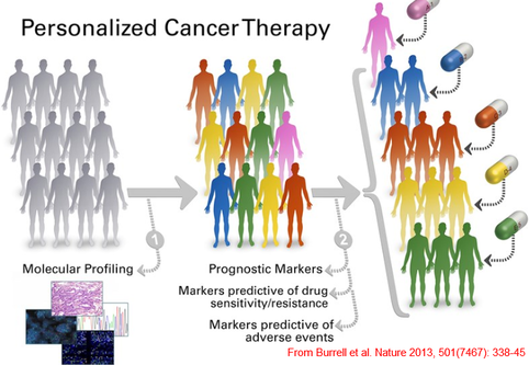 Why is personalised medicine a different approach? Personalised medicine is a paradigm shift: from the quest of a treatment that will fit most of the patients, the aim is now to tailor treatments to the patient’s medical history, personal “parameters” (age, gender...), environment, even microbiome (one’s microbial population might be as unique as one’s fingerprints [1]). Most of the diseases are diagnosed by looking at the phenotype but, sometimes, two sets of symptoms can overlap and characterising a disorder becomes complex. A more personalised approach can be useful as factors responsible for the phenotype (i.e symptoms) can differ and looking at individual factors could lead to easier characterisation thus better treatment of the disorder. Personalising is supposed to maximise the benefits and minimise side effects [2] but it is an ideal to pursue and in practice, available technologies and knowledges do not allow to fully achieve it. Nonetheless, research to personalize medicine offers fascinating examples and, in the oncology field in particular, allows new tumour classifications, first step towards a complete personalised characterisation. Here is outlined what can be done in oncology thanks to these new technologies. One important part of the personalised medicine is the genomic medicine [3] i.e the medicine that tries to extract information from genomes (structural genomics) or from transcriptomes/proteomes/epigenomes (functional genomics). Such approach is now possible because of the Next Generation Sequencing that allows a higher throughput (i.e the number of nucleobases read by run by day)and oncology benefited from this huge leap forward. Characterising tumours is like taking measurements for a custom-made tuxedo: Cancers used to be characterized by an organ-based classification [2] but genetic analysis allowed to discover that cancers resulted from an accumulation of mutations and some of those mutations were found within many neoplastic tissues: an organ-based classification became obsolete. Moreover, tumours are composed of several sub-clonal populations and healthy cells that interact so there is intra-heterogeneity (differences within the same tumour). Finally, two patients with the same tumour location can have different subclones so there is inter-heterogeneity (differences between two individual tumours from the same type) too. 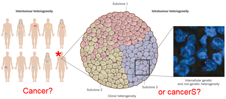 Alexandrov et al. [4] studied 4,938,362 mutations from 7, 042 cancers and that ideally allows to look for two things:
Describing is a start… But predicting matters too: There was an important word in the previous sentence. Until now, we only saw how genetic analyses allow to characterise a disorder: this is the diagnosis. BUT! One aim of a personalised treatment is also to PREDICT. How can we do that in practice is one of the subjects of my internship on gliomas and can be briefly explained step-by-step: i) two types of tumours are studied to study the prognostic variation; ii) two genes are studied with one that is known to be frequently found in those tumours or known to play a role in the tumorigenesis and the second one that will help to categorise; iii) correlations between clinical and genetic observations: patients are separated into several groups according to their mutation status and clinical data are coupled to each group. For example, if patients with genes A and B mutated live longer than those with A mutated and normal B, clinicians will be able to predict the disease evolution in other patients with known mutation status. Another interest: if a specific mutation-status-associated phenotype is known to be susceptible to react to a drug, a mutated patient can be treated with it (crucial when we know chemotherapeutic side effects). Now you know! What is the take-home message? First, new sequencing technologies allow to study diseases from another point of view and to open new therapeutic windows. Second, the more precisely a disease is characterised, the more tailored the treatment can be and this is why personalised medicine development is tightly correlated to genetic advances. Third, personalised medicine is in its infancy: a completely tailored treatment is rare and one limitation is that personalised treatments must also take into account the resistance that can arise (for example, radiotherapy in cancer selects the strongest phenotypes and in many cases of recurrence, the tumour is less likely to be destroyed) and the evolution of the disease so medicine will truly be personalised when we will understand better how disorders work. Finally, even if it is the beginning, personalised medicine allows to improve diagnosis/prognosis in several fields including cancer by taking the first step before a complete individual characterisation: the stratification of the patients into risk/prognostic groups. REFERENCES, in case you’d like to learn more: [1] Franzosa, E., Huang, K., Meadow, J., Gevers, D., Lemon, K., Bohannan, B. and Huttenhower, C. (2015). “Identifying personal microbiomes using metagenomic codes”. Proceedings of the National Academy of Sciences, 112(22), pp.E2930-E2938. [2] Ogino, Shuji et al. “Cancer Immunology—Analysis Of Host And Tumor Factors For Personalized Medicine”. Nature Reviews Clinical Oncology 8.12 (2011): 711-719. Web. 8 Jan. 2017. [3] Ginsburg, Geoffrey S. and Huntington F. Willard. "Genomic And Personalized Medicine: Foundations And Applications". Translational Research 154.6 (2009): 277-287. Web. 8 Jan. 2017. [4] Alexandrov, Ludmil B. et al. "Signatures Of Mutational Processes In Human Cancer". Nature 500.7463 (2013): 415-421. Web. 8 Jan. 2017. [5] Boisselier, B., Gallego Perez-Larraya, J., Rossetto, M., Labussiere, M., Ciccarino, P., Marie, Y., Delattre, J. and Sanson, M. (2012). “Detection of IDH1 mutation in the plasma of patients with glioma”. Neurology, 79(16), pp.1693-1698. [6] Hanahan, Douglas and Robert A. Weinberg. "Hallmarks Of Cancer: The Next Generation". Cell 144.5 (2011): 646-674. Web. |
Search the site...
Photo used under Creative Commons from DJANDYW.COM & DJANDYW.TV AKA ANDREW WILLARD
